Lets go show

시스템 환경

Hardware Resources : CPU 8 Core, 4GB Memory

Test Tool : k6 

Mornitoring Tool : Prometheus , Grafana

Application : Spring Boot Application (Boot Version 3.2.5)

DB : Mysql 

모니터링 환경

- K6 에서 조금 더 세세한 정보를 수집하기 위해서 InfluxDB + Grafana 연동

- SpringBoot Application 관련 메트릭 정보 수집을 위해 SpringBoot Actuator + Prometheus + Grafana 연동

- 시스템 메트릭 수집을 위해 Node Exporter + Prometheus + Grafana 연동

테스트 시나리오

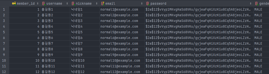
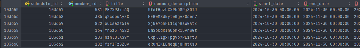
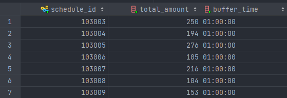
- 약 40만개의 일정 데이터로 테스트를 진행했습니다. (일정 = 고정일정 + 변동일정 + 일반일정 ) 

   본 테스트에서는 일반일정 데이터는 거의 추가하지 않고 (약 1만개) 고정일정 + 변동일정 데이터만 추가하여 진행했다.

- 일정관리 웹 서비스로써 일정조회에 대한 요청이 대다수 일 것이라고 판단하고 테스트를 진행했다. 

- 테스트 시나리오는 일정 조회 Api 에 Virtual User를 활용하여 Get 요청을 보내 유저의 최근 3개월 내 모든 일정을 조회한다.

- 응답시간 목표를 95% 이상의 요청은 500ms 이하로 설정했다.

- CPU사용량, Memory 사용량  P95~P99 응답시간, TPS , 에러율 등을 고려하여 부하를 판단했다.

- IntelliJ Profiler , (디비 수준에서의 병목 쿼리 파악하기.) 병목 지점을 파악했다.

1. 성능 테스트

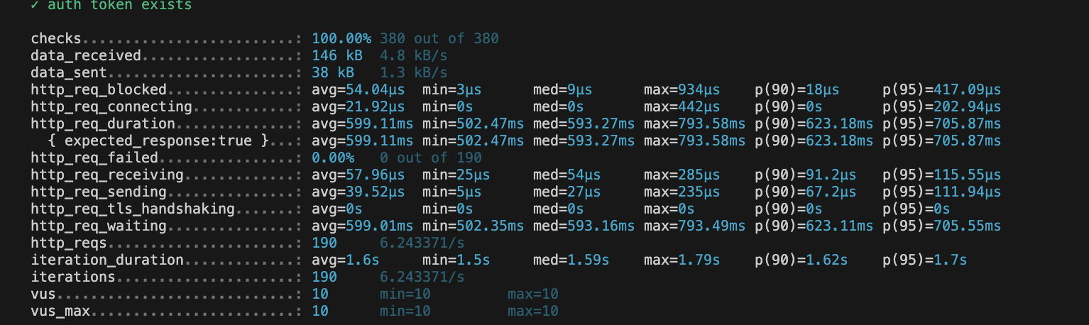
먼저 시스템의 임계점을 분석하기 위해 스트레스 테스트를 진행했고,  0명의 가상 유저부터 70명의 가상유저까지 점차적으로 늘리는 Ramping-vus 방식으로 테스트를 진행했다. 

Virtual User의 수가 약 40명 정도 부근에 가까워 졌을때 부터 지연율이 높아졌으며 p95 기준 응답시간 목표인 500ms 보다 더 늦은약 500ms~1s 사이의 응답 시간을 보여 주었다. 그렇기 때문에 해당 지점을 임계치를 초과한 지점으로 보고 45Vus 를 유지한 상태에서 부하테스트를 진행하였고 결과 역시나 성능이 좋지 않음을 확인할 수 있었다.

2. 병목 지점 파악

Spring Profiler

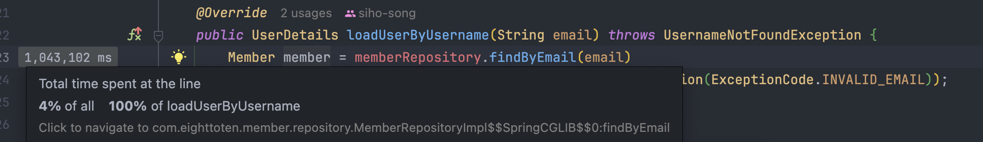
부하 테스트 이후 먼저 Spring profiler를 통해 실행결과를 확인했다.

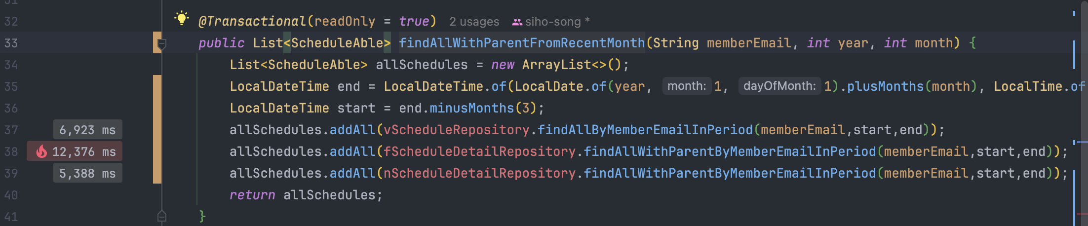
 다음은 일정 조회시 조회 시나리오에 맞게 분석한 결과이다.

- 1. memberRepository.find - 단순 조회

- 2. vScheduleRepository.find - 단순 조회 

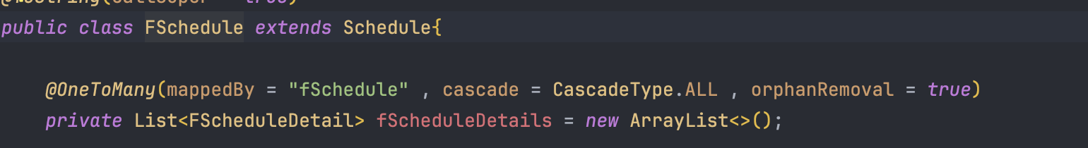
- 3. fScheduleDetailRepository.find - 1번의 left join

- 4. nScheduleDetailRepository.find - 1번의 left join

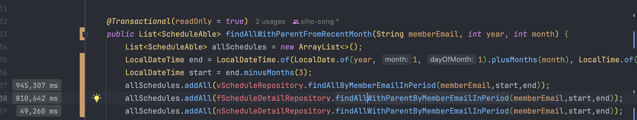
위 결과에서 확인할 수 있는건 cpu 사용시간에 비해 전체 실행시간이 훨씬 길다는 것을 확인할 수 있었다. 즉 전체 실행 시간 대비 CPU Time이 매우 적으므로, 대부분의 시간은 I/O 대기 시간이라고 볼 수 있다.

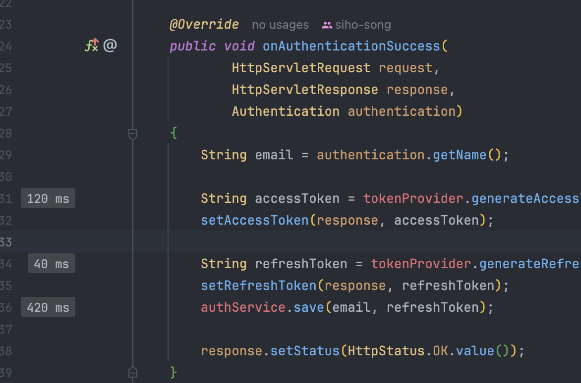
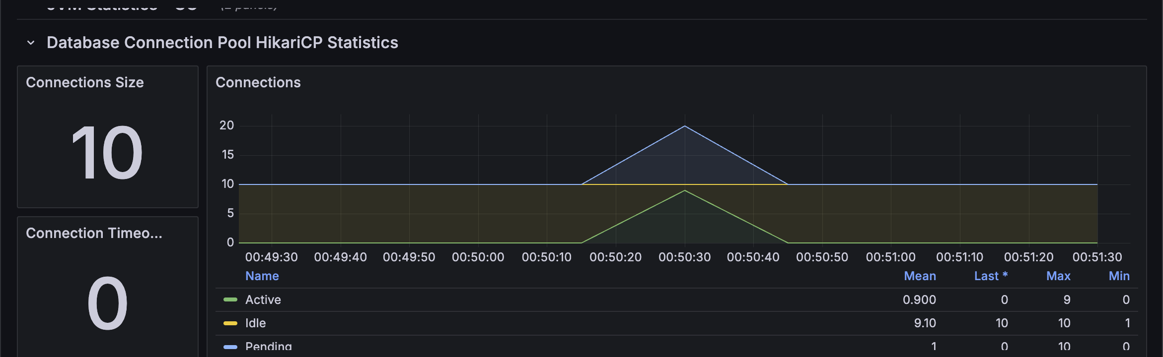
 추가적으로 Hikary CP 의 커넥션을 확인해 보면 모든 커넥션이 사용중이고, 평균 9개에서 최대 15개의 요청이 커넥션을 얻기 위해 대기중이라는 것을 확실히 확인할 수 있었다. 그렇기 때문에 DB에서의 병목을 파악해서 위 문제를 해결하고자 했고 쿼리 실행 계획을 활용해서 위 시나리오들의 각 쿼리들에 대해서 분석해보았다. 

1. EXPLAIN ANALYZE SELECT * FROM member WHERE email = 'normal1@example.com';

Res) -> Rows fetched before execution  (cost=0..0 rows=1) (actual time=251e-6..293e-6 rows=1 loops=1)

2. EXPLAIN ANALYZE SELECT *  FROM v_schedule  WHERE start_date_time >= '2025-01-01 00:00:00'    AND end_date_time <= '2025-03-08 23:59:59'    AND created_by = 'normal1@example.com'	

Result) Filter: ((v_schedule.created_by = 'normal1@example.com') and (v_schedule.start_date_time >= TIMESTAMP'2025-01-01 00:00:00') and (v_schedule.end_date_time <= TIMESTAMP'2025-03-08 23:59:59'))  (cost=20367 rows=2199) (actual time=0.229..126 rows=2 loops=1)
    -> Table scan on v_schedule  (cost=20367 rows=197977) (actual time=0.209..108 rows=199999 loops=1)
    
    
3. EXPLAIN ANALYZE SELECT *  FROM f_schedule_detail fd left outer join f_schedule f on f.f_schedule_id = fd.f_schedule_id WHERE fd.start_date_time >= '2025-01-01 00:00:00'    AND fd.end_date_time <= '2025-03-08 23:59:59'    AND fd.created_by = 'normal1@example.com'	

Res) Nested loop left join  (cost=18427 rows=1923) (actual time=0.213..117 rows=35 loops=1)
    -> Filter: ((fd.created_by = 'normal1@example.com') and (fd.start_date_time >= TIMESTAMP'2025-01-01 00:00:00') and (fd.end_date_time <= TIMESTAMP'2025-03-08 23:59:59'))  (cost=17754 rows=1923) (actual time=0.124..117 rows=35 loops=1)
        -> Table scan on fd  (cost=17754 rows=173117) (actual time=0.114..99.2 rows=175000 loops=1)
    -> Single-row index lookup on f using PRIMARY (f_schedule_id=fd.f_schedule_id)  (cost=0.25 rows=1) (actual time=0.00294..0.00298 rows=1 loops=35)
    
4. EXPLAIN ANALYZE SELECT *  FROM n_schedule_detail nd left outer join n_schedule n on n.n_schedule_id = nd.n_schedule_id WHERE nd.start_date_time >= '2025-01-01 00:00:00'    AND nd.end_date_time <= '2025-03-08 23:59:59'    AND nd.created_by = 'normal1@example.com'

Res) -> Nested loop left join  (cost=666 rows=64.8) (actual time=9.46..9.46 rows=0 loops=1)
    -> Filter: ((nd.created_by = 'normal1@example.com') and (nd.start_date_time >= TIMESTAMP'2025-01-01 00:00:00') and (nd.end_date_time <= TIMESTAMP'2025-03-08 23:59:59'))  (cost=607 rows=64.8) (actual time=9.46..9.46 rows=0 loops=1)
        -> Table scan on nd  (cost=607 rows=5829) (actual time=0.107..8.11 rows=5963 loops=1)
    -> Single-row index lookup on n using PRIMARY (n_schedule_id=nd.n_schedule_id)  (cost=0.814 rows=1) (never executed)

1번의 경우 이미 유니크 키로 지정되어있는 유저의 email을 기준으로 index가 생성되어 있기때문에 매우 빠른시간내에 조회하고 있다는 점을 확인할 수 있었다.

2번,3번,4번 같은 경우는 join 대상이 되는 테이블같은 경우는 PK 인덱스를 통해 빠르게 조회가 되는 것을 확인할 수 있지만 자기 테이블에 대해서는 인덱스 없이 Full-Scan 하고 있었기 때문에 적절한 인덱스를 생성하여 조회 시간을 감축시킬 수 있다고 생각했다. 

각 일정들의 조회를 동반하는 쿼리 중 id로 조회하는걸 제외하면 start_date_time, created_by를 기준으로 조회를 하는 경우가 대다수이고 거의 대부분의 시나리오에서 위와 같은 모든 일정을 start_date_time, end_date_time 사이의 일정을 조회하기 때문에start_date_time, end_date_time,created_by 에 대해서 복합 인덱스를 생성하는 것이 좋을 것이라 판단했다.

3. Index 적용

인덱스를 설계한다고 했을 때, start_date_time,end_date_time,created_by 순으로 인덱스를 설계한다고 가정하면 첫 번째 컬럼이 범위 검색이므로 인덱스가 제대로 작동하지 않을 수 있다고 생각했고 실제로도 그랬다. 따라서 (created_by, start_date_time, end_date_time) 의 복합 인덱스를 생성했다.

고정일정 인덱스 적용 후 

Nested loop left join  (cost=22.5 rows=35) (actual time=0.14..0.311 rows=35 loops=1)
    -> Index range scan on fd using f_detail_created_start_end_idx over (created_by = 'normal1@example.com' AND '2025-01-01 00:00:00' <= start_date_time), with index condition: ((fd.created_by = 'normal1@example.com') and (fd.start_date_time >= TIMESTAMP'2025-01-01 00:00:00') and (fd.end_date_time <= TIMESTAMP'2025-03-08 23:59:59'))  (cost=16 rows=35) (actual time=0.0772..0.223 rows=35 loops=1)
    -> Single-row index lookup on f using PRIMARY (f_schedule_id=fd.f_schedule_id)  (cost=0.259 rows=1) (actual time=0.00219..0.00223 rows=1 loops=35)

변동일정 인덱스 적용 후 

Index range scan on v_schedule using v_schedule_created_start_end_idx over (created_by = 'normal1@example.com' AND '2025-01-01 00:00:00' <= start_date_time <= '2025-03-08 23:59:59'), with index condition: ((v_schedule.created_by = 'normal1@example.com') and (v_schedule.start_date_time between '2025-01-01 00:00:00' and '2025-03-08 23:59:59'))  (cost=1.16 rows=2) (actual time=0.0883..0.112 rows=2 loops=1)


일반일정 인덱스 적용 후

Nested loop left join  (cost=1.08 rows=1) (actual time=0.0591..0.0591 rows=0 loops=1)
    -> Index range scan on nd using n_detail_created_start_end_idx over (created_by = 'normal1@example.com' AND '2025-01-01 00:00:00' <= start_date_time), with index condition: ((nd.created_by = 'normal1@example.com') and (nd.start_date_time >= TIMESTAMP'2025-01-01 00:00:00') and (nd.end_date_time <= TIMESTAMP'2025-03-08 23:59:59'))  (cost=0.71 rows=1) (actual time=0.0581..0.0581 rows=0 loops=1)
    -> Single-row index lookup on n using PRIMARY (n_schedule_id=nd.n_schedule_id)  (cost=1.11 rows=1) (never executed)

4. Index 적용 후 비교

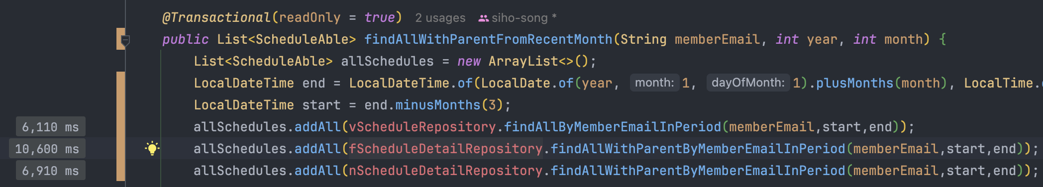
Index 적용 후 적용 전과 같은 조건으로 테스트를 진행했다. 

Spring Profiler 로 비교

Index 적용 전과 CPU 사용시간은 크게 다르지 않은 것을 확인할 수 있다. 그리고 전체 실행시간은 약 180만 ms -> 약 6만 ms 로 감축된 것을 확인할 수 있다.

HikariCP의 Connection 사용 또한 처음 동시접속이 있었을때 pending 상태 이후로는 안정적으로 처리하는 것을 확인할 수 있었다.

또한 Grafana를 통해 확인해보면 req_duration (p95) 기준으로 4.94(4940ms)초에서 57.10ms 로 약 86배 줄어든 것을 확인할 수 있다.

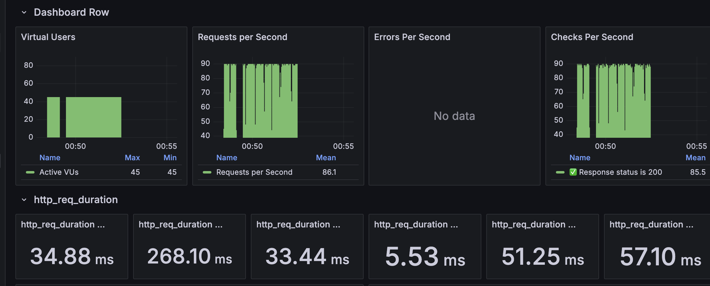
위와 같이 성능 개선을 확인하고 Virture User의 수를 늘려서 추가적으로 스트레스 테스트를 진행해보았다.

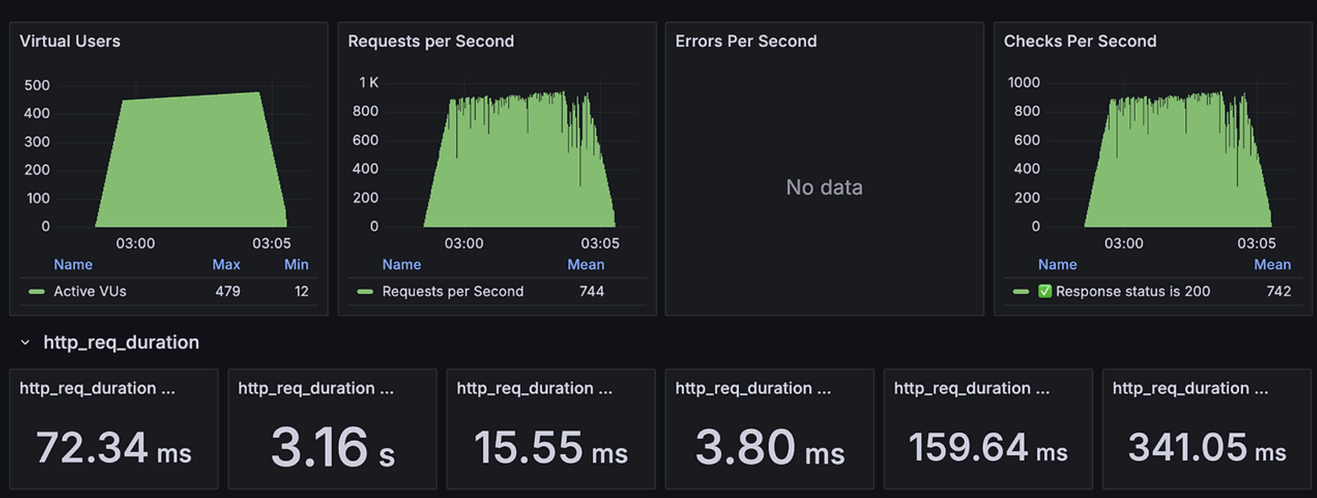
RPS(Requests Per Seconds)가 23에서 744로 약 32배 증가하여 처리량이 크게 개선되었음을 확인할 수 있다. 추가적인 개선은 시스템의 메모리와 CPU 사용량을 모니터링하고 적절량 만큼의 HikariCP 의 max_pool_size를 늘린다면 추가적인 성능 개선이 가능 할 것 같 DB 레벨에서의 지연이 어플리케이션에 얼마나 큰 영향을 미치는지 실감할 수 있었다.

현재 진행하고 있는 프로젝트의 멀티 모듈화를 마치고 해당 글을 작성하여 글의 내용에 누락이 있을 수 있다는 점에 대해 양해를 부탁드립니다. 

프로젝트 설명

먼저 프로젝트에 관해 간단하게 설명하자면 8to10 이라는 이름의 갓생을 살고자하는 P 성향의 사람에게 세우기 귀찮은 계획을 세워주며 일정 수행을 어느정도 강제하기 위해 진행한 일정관리 프로젝트이다.
프로젝트를 진행할 때 기업이 운영하는 정도의 대규모 어플리케이션 정도로 설계하는 것은 불가능 하겠지만 사용자가 많은 어플리케이션의 상황을 어느정도 가정하고 설계하려고 했다. 그렇기 때문에 설계적 관점과 유지보수 측면에서의 관점 둘다에 대해서 고려할 필요가 있었다.

아래는 해당 프로젝트의 아키텍처 자료이다.

요약하자면 1개의 클러스터 3개의 pod로 AutoScaling되는 분산서버, 단일 db, 단일 캐시로 구성된 아키텍처이다.

멀티 모듈화의 이유

1. Scheduling 서버의 분리
   서비스의 기능 중 정해진 시간에 사용자에게 알람으로 하나의 피드백 메시지를 날려주는 스케쥴링 서비스를 필요로 한다.
   하지만 위 구조에서 3개의 서버가 중복된 피드백 메시지를 동일 사용자에게 전송하는 문제가 있었다. 그렇기 때문에 Scheduling 서버에 대한 분리가 필요했다.
2. 멀티 모듈화로 얻을 수 있는 추가적인 이점들
   • 테스트 코드 구현시 테스트 환경의 분리
   • 변경된 모듈만 개별적으로 빌드 및 배포 가능
   • 등등

멀티 모듈화를 생각하게 되었던 가장 큰 이유는 Scheduling 서버의 분리 때문이었다.  Scheduling 서버의 분리 이외에도 멀티 모듈화를 진행하면서 얻을 수 있는 부수적인 장점도 많았다. 모듈화를 진행하는 과정에서 여러가지에 대해 고민을 하면서 단순히 기존의 코드를 분리하는 것이 아니라 도메인객체와 엔티티 객체를 분리하고 도메인 객체를 바라보는 관점과 레이어를 바라보는 관점 그리고 테스트 코드를 다시 작성하고 기존의 코드를 수정하는 과정에서  많은 부분을 배울 수 있었다. 그렇기에 나의 고민과 진행 과정을 시리즈 글로 남기려고 하고 이 글을 보는 사람들과 다양한 생각을 나눌수 있으면 좋을 것 같다.

이번 글에서는 내가 했던 gradle 세팅에 대해 작성하고자 한다.

Gradle 세팅 및 모듈 추가

기존 gradle 구성

build.gradle

dependencies {
    implementation 'org.springframework.boot:spring-boot-starter-aop'
    implementation 'org.springframework.boot:spring-boot-starter-data-jpa'
    implementation 'org.springframework.boot:spring-boot-starter-validation'
    implementation 'org.springframework.boot:spring-boot-starter-web'

    implementation 'org.springframework.boot:spring-boot-starter-actuator'

    //redis
    implementation 'org.springframework.boot:spring-boot-starter-data-redis'

    // spring security
    implementation 'org.springframework.boot:spring-boot-starter-security'

    implementation 'com.mysql:mysql-connector-j'
    // jwt
    implementation 'io.jsonwebtoken:jjwt-api:0.11.5'
    runtimeOnly 'io.jsonwebtoken:jjwt-impl:0.11.5'
    runtimeOnly 'io.jsonwebtoken:jjwt-jackson:0.11.5'

    //json
    implementation 'org.json:json:20231013'

    compileOnly 'org.projectlombok:lombok'
    annotationProcessor 'org.projectlombok:lombok'

    // P6Spy 의존성 추가 (개발 서버용)
    implementation 'p6spy:p6spy:3.9.1'

    //Querydsl 추가
    implementation 'com.querydsl:querydsl-jpa:5.0.0:jakarta'
    annotationProcessor "com.querydsl:querydsl-apt:${dependencyManagement.importedProperties['querydsl.version']}:jakarta"
    annotationProcessor("jakarta.persistence:jakarta.persistence-api")
    annotationProcessor("jakarta.annotation:jakarta.annotation-api")

    testImplementation 'org.springframework.boot:spring-boot-starter-test'
    testImplementation 'org.springframework.security:spring-security-test'
    testImplementation 'com.h2database:h2'
    testImplementation 'com.github.codemonstur:embedded-redis:1.4.3'

    //parametererized test
    testImplementation 'org.junit.jupiter:junit-jupiter-params'
    testCompileOnly 'org.projectlombok:lombok'
    testAnnotationProcessor 'org.projectlombok:lombok'
}

위 gradle 세팅을 보면 여러 역할을 하는 implementation 구문들이 쌓여있는 것을 확인할 수 있다. 이는 해당 모듈이 정확히 어떤일을 하고 있는지 파악하기 힘들게 만들고, 하나의 기능에 대한 변경이 다른 코드에 대해 영향을 미칠 수 있다는 것을 뜻한다. 

settings.gradle

    rootProject.name = 'eighttoten'

패키지 구조

기존의 패키지 구조는 다음과 같다.

현재 패키지의 구조를 보면 achivement라는 도메인 관련 패키지 하위에 모든 레이어의 코드들이 혼재되어 있는 상태이지만 data access와 관련된 코드들은 data access 와 관련된 모듈안에 모여있는 것이, 다른 계층도 마찬가지로 관련된 기능들이 같은 모듈안에 모여있는 것이 더 응집도 측면에서 잘 응집되어 있는 것이 아닐까 라는 생각이 든다. 이 기능들을 관심사에 맞게 차근차근 하나씩 분리하고자 한다.

아래는 이를 위해 공통적으로 해야할 gradle 세팅들에한 내용이다.

1. 기존의 settings.gradle 상위 폴더로 빼주고 다음과 같이 변경했다.

`rootProject.name = 'eighttoten'`

include(  
"8to10_backend"  
)

위 설정을 통해 프로젝트에서 8to10_backend 모듈을 include 할 수 있게 된다. 

2. 기존의 build.gradle 파일을 상위 폴더에 복사 붙여넣기 한다.

해당 파일을 상위에 생성하는 이유는 공통 implementation이나 프로젝트 세팅을 위해서 이다. 아직은 하나의 모듈만 있기때문에 복사 붙여넣기 했다. 

3. 모듈들의 공통 버전 관리를 위해 gradle.properties 파일을 상위 폴더에 생성한다.

이렇게 gradle.properties 파일을 생성함으로써 각 버전들에 대한 변수를 정의하고 하나의 파일에서 모듈들의 버전에 대해 통합적으로 관리할 수 있다.

### Application Version ###
applicationVersion=0.0.1

### Project configs ###
projectGroup=online.8to10

javaVersion=17

springBootVersion=3.2.5
springDependencyManagementVersion=1.1.4

4. settings.gradle 수정

settings.gradle 에서 서브 모듈들의 플러그인 버전을 관리 한다. 이렇게 중앙에서 플러그인을 관리함으로써 모듈들의 버전 충돌을 방지하고 유지보수성을 늘릴 수 있다.

pluginManagement {
    String springBootVersion = settings.getProperty("springBootVersion")
    String springDependencyManagementVersion = settings.getProperty("springDependencyManagementVersion")

    resolutionStrategy {
        eachPlugin {
            if (requested.id.id == "org.springframework.boot") {
                useVersion(springBootVersion)
            } else if (requested.id.id == "io.spring.dependency-management") {
                useVersion(springDependencyManagementVersion)
            }
        }
    }
}

5. 상위 폴더(아까 복사 붙여넣기 했던) build.gradle 수정

plugins {
    id 'java'
    id 'org.springframework.boot' apply false
    id 'io.spring.dependency-management' apply false
}

configurations {
    compileOnly {
        extendsFrom annotationProcessor
    }
}

allprojects {
    java.sourceCompatibility = javaVersion
    group = projectGroup
    version = applicationVersion

    repositories {
        mavenCentral()
    }
}

subprojects {
    apply plugin: 'java'
    apply plugin: 'org.springframework.boot'
    apply plugin: 'io.spring.dependency-management'

    dependencies {
        implementation 'org.springframework.boot:spring-boot-starter-aop'
        implementation 'org.springframework.boot:spring-boot-starter-data-jpa'
        implementation 'org.springframework.boot:spring-boot-starter-validation'
        implementation 'org.springframework.boot:spring-boot-starter-web'

        implementation 'org.springframework.boot:spring-boot-starter-actuator'

        //redis
        implementation 'org.springframework.boot:spring-boot-starter-data-redis'

        // spring security
        implementation 'org.springframework.boot:spring-boot-starter-security'

        implementation 'com.mysql:mysql-connector-j'
        // jwt
        implementation 'io.jsonwebtoken:jjwt-api:0.11.5'
        runtimeOnly 'io.jsonwebtoken:jjwt-impl:0.11.5'
        runtimeOnly 'io.jsonwebtoken:jjwt-jackson:0.11.5'

        //json
        implementation 'org.json:json:20231013'

        compileOnly 'org.projectlombok:lombok'
        annotationProcessor 'org.projectlombok:lombok'

        // P6Spy 의존성 추가 (개발 서버용)
        implementation 'p6spy:p6spy:3.9.1'

        //Querydsl 추가
        implementation 'com.querydsl:querydsl-jpa:5.0.0:jakarta'
        annotationProcessor "com.querydsl:querydsl-apt:${dependencyManagement.importedProperties['querydsl.version']}:jakarta"
        annotationProcessor("jakarta.persistence:jakarta.persistence-api")
        annotationProcessor("jakarta.annotation:jakarta.annotation-api")

        testImplementation 'org.springframework.boot:spring-boot-starter-test'
        testImplementation 'org.springframework.security:spring-security-test'
        testImplementation 'com.h2database:h2'
        testImplementation 'com.github.codemonstur:embedded-redis:1.4.3'

        //parametererized test
        testImplementation 'org.junit.jupiter:junit-jupiter-params'
        testCompileOnly 'org.projectlombok:lombok'
        testAnnotationProcessor 'org.projectlombok:lombok'
    }

    def generated = 'src/main/generated'

    // querydsl QClass 파일 생성 위치를 지정
    tasks.withType(JavaCompile) {
        options.getGeneratedSourceOutputDirectory().set(file(generated))
    }

    // java source set 에 querydsl QClass 위치 추가
    sourceSets {
        main.java.srcDirs += [ generated ]
    }

// gradle clean 시에 QClass 디렉토리 삭제
    clean {
        delete file(generated)
    }

    tasks.named('test') {
        useJUnitPlatform()
    }

    tasks.getByName("bootJar"){
        enabled = false
    }

    tasks.getByName("jar"){
        enabled = true
    }
}

위와 같이 apply 를 적용함으로 써 특정 서브 모듈에서 필요한 플러그인은 해당 서브 모듈에서 따로 정의하여 적용할 수 있다. 현재는 모듈이 하나밖에 없기 때문에 기존의 플러그인을 그대로 submodule에 적용해놓은 상태이다. 최종적으로 build.gradle 파일에서 dependency 관련 설정 빼고는 버전에 관련된 모든 숫자가 제거된 것을 확인할 수 있다. 

Reference) https://www.youtube.com/results?search_query=%EC%A0%9C%EB%AF%B8%EB%8B%88%EC%9D%98+%EA%B0%9C%EB%B0%9C%EC%8B%A4%EB%AC%B4

개인 프로젝트에서 진행했던 알람 시스템 구현에 대해서 포스팅 하려한다. 

알람 시스템을 구현하기 위해서는 서버의 알람 이벤트를 클라이언트에게 전송할 수 있어야 하는데  이 때 고려했던 방법은 SSE 연결과 웹소켓을 이용한 연결이었다. 알람 전송을 위해서는 단방향 전송이 필요했기 때문에 SSE 연결을 통해 알람 기능을 구현하고자 했다. 

알람 구독 시나리오는 다음과 같다. 클라이언트 사이드에서는 javascript 가 제공하는 eventsource 객체를 통해 서버의 /subscribe 로 연결 요청을 보내고 연결을 맺는다. 서버에서는 in-memory 방식으로 해당 클라이언트의 연결정보를 관리하면서 연결을 유지한다. 아래는 클라이언트와 서버와 Sse 연결을 맺는 기본 구현 코드이다. 

@GetMapping(value = "/subscribe", produces = MediaType.TEXT_EVENT_STREAM_VALUE)
public ResponseEntity<SseEmitter> subscribe(
        @CurrentMember Member member,
        @RequestHeader(value = "Last-Event-ID", required = false) String lastEventId) {
    return ResponseEntity.ok(sseEmitterService.subscribe(member, lastEventId));
}

public SseEmitter subscribe(Member member, String lastEventId) {
    SseEmitter emitter = new SseEmitter(DEFAULT_TIMEOUT);
    String uniqueEmitterId = generateUniqueClientId(member.getEmail(),LocalDateTime.now());
    sseEmitterRepository.save(uniqueEmitterId, emitter);

    emitter.onCompletion(() -> sseEmitterRepository.deleteById(uniqueEmitterId));
    emitter.onTimeout(() -> sseEmitterRepository.deleteById(uniqueEmitterId));
    emitter.onError((e) -> sseEmitterRepository.deleteById(uniqueEmitterId));

    sendToClient(emitter,uniqueEmitterId,"init","init");

    if(lastEventId != null){
        LocalDateTime dateTime = extractDateTime(lastEventId);
        List<Notification> notifications = notificationService.findAllAfterDateTime(dateTime, member);
        notifications.forEach(
                notification -> sendToClient(emitter,
                        uniqueEmitterId,
                        "notification",
                        NotificationResponse.from(notification))
        );
    }

    return emitter;
}

public void sendToClient(SseEmitter emitter, String id, String name, Object data) {
    try {
        emitter.send(
                SseEmitter.event()
                        .id(id)
                        .name(name)
                        .data(data)
        );
    } catch (IOException e) {
        log.error(e.getMessage(), e);
        sseEmitterRepository.deleteById(id);
        throw new RuntimeException(FAILED_SSE_NOTIFICATION_SEND.getMessage());
    }
}

@Repository
public class SseEmitterRepository {
    private Map<String, SseEmitter> emitterMap = new ConcurrentHashMap<>();

    public List<SseEmitter> findAllStartWithByMemberEmail(String email) {
        return emitterMap.entrySet().stream()
                .filter(entry-> entry.getKey().startsWith(email))
                .map(Entry::getValue)
                .toList();
    }

    public SseEmitter save(String id, SseEmitter emitter) {
        return emitterMap.put(id, emitter);
    }

    public void deleteById(String uniqueEmitterId) {
        emitterMap.remove(uniqueEmitterId);
    }

    public void deleteAll(){
        emitterMap.clear();
    }
}

톰캣의 쓰레드풀에 있는 각 쓰레드당 하나의 연결 요청을 처리하기 때문에 공유 자원에 대한 경쟁상황이 생길 수 있으므로

ConcurrentHashMap을 사용하여 SseEmitter 객체를 관리한다. 

해당 프로젝트에서 알람이 발생하는 상황은 다음과 같다.

•  A유저의 게시글에 B 유저가 댓글을 달았을 때
•  A유저의 댓글에 B 유저가 대댓글을 달았을 떄
• Todo 업데이트 마감 시간 공지
• 새벽 1시 각 유저에게 성취도 피드백 메시지 공지 

단일서버에서 1번 상황이 발생했다고 가정했을 때는 모든 요청이 하나의 서버로만 전달 되기때문에 해당 서버는 반드시 알람 구독을 맺고있는 클라이언트의 정보를 갖고 있을 것이다. 그렇기 때문에 A의 게시글에 B 의 댓글이 등록될 때 댓글 등록 이벤트를 발생시키고 이벤트 리스너에서 해당 이벤트를 수신하여 A에게 알람을 전송하면 문제가 없다. 

하지만 본 프로젝트는 단일서버가 아닌 Scale-out 된 분산서버 환경을 고려하고 설계하였기 때문에 서버가 여러개인 상황을 가정하면, 댓글 등록 이벤트를 발생시킨 서버에서 A유저의 연결정보가 서버에 존재한다고 보장할 수 없다. 왜냐하면 DB에 따로 연결정보를 관리하지 않고 in-memory 형식으로 연결정보를 관리하고 있기 때문이다. 

그렇기 때문에 댓글 등록 이벤트가 발생했을 때 A의 연결정보를 갖고 있는 서버에서 댓글 등록 이벤트를 처리하고 알림을 전송할 수 있도록 하는 구조설계가 필요했다. 

위와 같은 이유로 Kafka 를 통한 Producer-Consumer 그리고 Redis Pub/Sub 두가지를 고려했다. Kafka 는 토픽을 구독하는 컨슈머 그룹내에 하나의 컨슈머가 토픽에 발행된 메시지를 처리하게 되는데 이 때 해당 컨슈머가 A의 연결정보를 가지고 있다라고 보장할 수 없는 상황이긴 마찬가지였다. 그렇기 때문에 채널을 구독하고 있는 모든 Subcriber가 메시지를 수신하고 해당 메시지를 처리할 수 있는 서버(Subscriber)에서 알람 전송을 처리할 수 있는 구조인 Redis Pub/Sub 구조를 채택하게 되었다. 

먼저 레디스 채널에 전송할 Event 객체를 구현했다.

public class NotificationEvent {
    String clientEmail;
    Long targetEntityId;
    Long relatedEntityId;
    String message;
    NotificationType notificationType;
}

각 필드에 대한 설명

1. SseEmitter 객체를 찾을때 clientEmail을 기반으로 연결을 찾도록 설계하였기 때문에 clientEmail 을 필드로 갖는다.

2. targetEntityId - 게시글에 댓글이 달렸다면 해당 게시글의 id 를 필드로 갖는다

3. relatedEntityId - 게시글에 댓글이 달렸다면 해당 댓글의 id 를 필드로 갖는다.

4. message - 이벤트 발생상황에 맞는 메시지 

@Getter
public enum NotificationMessage {
    REPLY_ADD("회원님의 게시글에 댓글이 달렸어요 :) ") ,
    NESTED_REPLY_ADD("회원님의 댓글에 댓글이 달렸어요 :)"),
    TODO_UPDATE("잊지 않으셨죠 ? 투두 리스트 제출 마감 시간은 오후 11시 입니다 :)"),
    ;
    private final String message;

    NotificationMessage(String message) {
        this.message = message;
    }
}

5. NotificationType - 각 상황에 맞는 알림 타입

@Getter
public enum NotificationType {
    REPLY_ADD("댓글 추가", "/board",true),
    NESTED_REPLY_ADD("대댓글 추가", "/board", true),
    TODO_UPDATE("TODO 업데이트", null, true),
    ACHIEVEMENT_FEEDBACK("성취도", null, true),
    ;

    private final String value;
    private final String baseTargetUrl;
    private final Boolean isNeededSave;

    NotificationType(String value, String baseTargetUrl,Boolean isNeededSave) {
        this.value = value;
        this.baseTargetUrl = baseTargetUrl;
        this.isNeededSave = isNeededSave;
    }
}

1. 위 dto 객체를 생성하여 스프링의 EventPublisher를 통해 각 알림 타입에 맞는 이벤트를 비동기 발행한다. 해당 이벤트는 댓글이 생성될 때 발행하게 되는데 해당 이벤트의 발행이 댓글 생성 및 저장에 영향을 주어서는 안되고 동기적으로 처리될 필요가 없다고 생각했기 때문에 비동기처리 하였다. 

2. publishNotificationEvent 메서드에서 해당 이벤트를 수신하고 레디스 토픽("NotificationTopic")에 publish 한다.

3. 레디스 토픽을 구독하고 있는 서버에서 handleNotificationEvent 함수를 통해 토픽에 발행된 메시지를 수신하고 알람을 보낸다. 

@Async
public void publishReplyAddEvent(Board board, Reply reply) {
    Member boardWriter = board.getMember();
    Member replyWriter = reply.getMember();

    if(reply.getParent() != null){
        eventPublisher.publishEvent(new NotificationEvent(
                reply.getParent().getMember().getEmail(),
                board.getId(),
                reply.getId(),
                NotificationMessage.NESTED_REPLY_ADD.getMessage(),
                NotificationType.NESTED_REPLY_ADD));
    }

    if (!boardWriter.getEmail().equals(replyWriter.getEmail())) {
        eventPublisher.publishEvent(new NotificationEvent(
                boardWriter.getEmail(),
                board.getId(),
                reply.getId(),
                NotificationMessage.REPLY_ADD.getMessage(),
                NotificationType.REPLY_ADD));
    }

@Async
@EventListener
public void publishNotificationEvent(NotificationEvent event){
    try {
        String channelEvent = objectMapper.writeValueAsString(event);
        redisOperations.convertAndSend(notificationTopic.getTopic(), channelEvent);
    } catch (JsonProcessingException e) {
        log.error(e.getMessage(), e);
        throw new InvalidRedisMessageException(INVALID_REDIS_MESSAGE);
    }
}

public void handleNotificationEvent(String message) {
    NotificationEvent event = convertToObject(message, NotificationEvent.class);

    Member member = memberService.findByEmail(event.getClientEmail());

    Notification notification = Notification.from(member, event);
    if (notification.getNotificationType().getIsNeededSave()) {
        notificationService.save(notification);
    }

    List<SseEmitter> emitters = sseEmitterService.findAllStartWithByMemberEmail(member.getEmail());
    if (!emitters.isEmpty()) {
        String response = convertToJson(NotificationResponse.from(notification));
        emitters.forEach(emitter -> sseEmitterService.sendToClient(
                emitter,
                sseEmitterService.generateUniqueClientId(member.getEmail(), LocalDateTime.now()),
                NOTIFICATION_EVENT_NAME,
                response)
        );
    }
}

만약 SSE 연결이 끊겨있는 상황에서는 알람을 수신하지 못하기 때문에  알람을 RDB 에 저장해놓고 유저가 다시 SSE 연결을 맺었을 때 받지 못했던 알람을 수신할 수 있게 하였다. 구조를 개선하기 전 알람 기능의 문제는 결국 stateful 하게 설계되었기 때문에 발생하는 문제였고 stateless 하게 변경하면서 문제를 개선할 수 있었다.

결론은 알람이 이벤트가 어디에서 발생이 되어도 분산되어 있는 서버 중 처리할 수 있는 서버에서 알람을 처리할 수 있게 되었다.

사전 설정

build.gradle 의존성 추가

implementation 'org.springframework.boot:spring-boot-starter-aop'
implementation 'org.springframework.boot:spring-boot-starter-actuator'

application-dev.yaml 설정 추가

server:
  tomcat:
    mbeanregistry:
      enabled: true


 management:
     endpoints:
        health:
            show-details: always
        web:
            exposure:
                include: *

병목 지점 디버깅용 Aspect 추가 

Controller, Service , Repository Layer 각 함수 실행시간 로깅

@Aspect
@Component
@Slf4j
public class ExecutionTimeAspect {
    @Pointcut("execution(* com.eighttoten.service..*(..)) ||"
            + "execution(* com.eighttoten.controller..*(..)) ||"
            + "execution(* com.eighttoten.repository..*(..)))")
    public void businessLogicPointcut(){}

    @Around("businessLogicPointcut()")
    public Object loggingMethodExecutionTime(ProceedingJoinPoint joinPoint) throws Throwable {
        long start = System.currentTimeMillis();
        Object result = joinPoint.proceed();

        long executionTime = System.currentTimeMillis() - start;
        log.info("Method name : {} , executed in {} ms", joinPoint.getSignature(), executionTime);
        return result;
    }
}

로그인 시나리오 (로컬에서 테스트 진행) - k6 사용

- 10개의 동시요청을 19번 반복 (총 190번의 요청)

- 로컬에서 진행하였기 때문에 네트워크 병목은 거의 없다.

- p(95) 를 기준으로 705ms 정도 나오는것을 확인할 수 있었다. 

우선 로그인 시나리오는 다음과 같다.

POST localhost:8080/login -> EmailPasswordAuthenticationFilter -> CustomAuthenticationProvider -> MemberDetailsService.loadUserByUsername(조회 쿼리) -> AuthSuccessHandler -> authService.findByEmail(조회 쿼리) -> authRepository.save(쓰기 쿼리)

병목지점 찾기 

- 병목 지점을 찾기위해서 ExecutionTimeAspect 로 로깅 + Intellij Profiler 를 활용하여 실행시간 추가 로깅 

로깅을 해본 결과 BCryptPasswordEncoder.matches 메서드에서 전체 실행시간의 94프로를 차지하고 있는 것을 확인할 수 있었다. 

어플리케이션 설계상 해당 부분은 남겨두고 먼저 해결할 수 있는 부분에 집중하기로 했다.

해당 부분 병목에 비하면 작은 수준이지만 문제가 있는 부분은 refreshToken 저장을 위한 조회와 저장쿼리를 날린다는 것인데 즉 
유저 n명당 auth테이블에 접근하는 쿼리가 2개 발생하게 된다. 즉 n+1 문제가 발생하게 된다. 

이 부분을 해결하기 위해 고려한 방식은 위 테이블 구조처럼 물리적으로는 분리되어 있는 테이블 두개를 조인해서 Auth,Member를 필드로 갖는 Dto를 하나 만들어서 두개를 동시에 조회해서 사용하면 어떨까 라고 생각했는데 애초에 인증절차를 진행하는 부분과 , 인증 테이블에 인증객체를 넣어주는 방식이 분리되어 작동 하기 때문에 같은 트랜잭션에 소속될 수 없고 결국 조회쿼리를 한번 더 날려야하는 구조였기에 맞지 않다고 생각을 했다.

RefreshToken 자체가 유저가 로그인 할 때마다 매번 갱신되는 데이터이기도 하고 재인증 과정에서 자주 사용되는 데이터라는 점, saveOrUpdate시 조회,저장쿼리 모두 날리는 상황에서 하나의 쿼리로 처리할 수 있다는 부분에서 Auth 정보를 메모리에 저장하여 사용하는 방식을 택했다. 레디스 사용을 위한 구조 개선에 대한 코드는 본 포스트에서는 다루지 않겠다. 

Redis 적용전 (rps)

730ms (10개 동시요청 19번 반복 )

Redis 적용후

authService.save : 420ms (10개 동시요청 19번 반복)

위 케이스에서는 유저 1000명에 대해서 테스트를 진행했다. 드라마틱한 개선효과는 아니지만 아주 .. 약간의 개선은 이루어 졌지만 미미하다고 생각이 든다. 하지만 유저테이블에 인덱스가 걸려있지 않은 상황이고 유저의 수가 10만 -> 100만 혹은 더 많은 유저가 존재한다고 생각한다면 유저테이블을 풀스캔해야하고 선형적으로 조회 시간이 증가할 것이고 더 큰 개선효과가 생기지 않을까 생각해본다.

소규모 어플리케이션의 유저수를 기준으로 봤을 때는 성능 개선보다는 세션 저장을 위한 구조적인 이점을 가져수 있었다는 점이 더 크지 않을까 

실질적으로 문제를 해결하기 위해서는 bcrypt의 matches  연산이 cpu 집약적인 연산이기 때문에 cpu 코어를 늘려 가용가능한 쓰레드 수를 늘리거나 보다 실용적인 방법으로는 서버를 scale-out 하는 방법이 있을 것 같다. 

사용 Tools : SQL Procedure , Gatling

Tool 선정

개발 서버용 더미 데이터를 추가하기 위해 여러가지 툴을 검색해 보았다.

가장 간편하게 사용할 수 있는 방법을 위주로 보았는데 후보군에 Mockaroo, Procedure 가 있었다. Mockaroo 는 프로그래밍 코드 없이 쉬운 UI 로 간단하게 데이터를 생성할 수 있다는 장점이 있었는데 무료버전은 테스트 데이터를 한번에 1000rows 밖에 생성하지 못했고 비교적 더미데이터를 생성하는 쿼리 포맷자체도 간단했기에 Procedure를 작성하기로 했다.

데이터 생성 및 ERD

내가 생성하려는 데이터는 (게시글,게시글 좋아요, 게시글 스크랩) ,(댓글 및 대댓글, 댓글 좋아요), (변동일정), (고정일정,고정일정 세부사항), (일반일정,일반일정 세부사항),(유저, 유저의 auth 정보) 였다.

1. 유저 데이터 추가

Member 테이블 구조에 맞게 Procedure 를 작성했고 총 1000개의 더미 데이터를 삽입했다.

```sql
BEGIN
    DECLARE i INT DEFAULT 1;

    WHILE i <= 1000 DO
        INSERT INTO member (
            username, 
            nickname, 
            email, 
            password, 
            gender, 
            mode, 
            role, 
            image_file, 
            created_at, 
            created_by, 
            updated_at, 
            updated_by, 
            score, 
            phone_number, 
            auth_email, 
            auth_phone
        ) VALUES (
            CONCAT('홍길동', i), 
            CONCAT('닉네임', i), 
            CONCAT('normal', i, '@example.com'), 
            '$2a$12$vVyp1MKvgHaS68VKu/gyjeaFqHiXzKiu8Cq5A8jeoLZzHM900.0X2', 
            'MALE', -- 성별 예제 값 (M: 남성, F: 여성)
            'MILD', -- 모드 예제 값
            'NORMAL_USER', 
            NULL,
            NOW(), -- 생성 시간
            'ADMIN', -- 생성자
            NOW(), -- 업데이트 시간
            'ADMIN', -- 업데이트자
            FLOOR(RAND() * 100), -- 점수 (0~99 랜덤 값)
            CONCAT('011', LPAD(i, 8, '0')),
            false, 
            false 
        );
        SET i = i + 1;
END WHILE;
END

```

2. 인증 데이터 추가

 Auth 테이블 구조에 맞게 Procedure 를 작성했고 앞서 생성한 멤버 데이터와 1:1 매핑이 되는 1000개의 더미 데이터를 삽입했다.

```sql
BEGIN
    DECLARE i INT DEFAULT 1;

    WHILE i <= 1000 DO
        INSERT INTO AUTH (
            email, refresh_token, created_at, created_by, updated_at, updated_by
        ) VALUES (
            CONCAT('normal', i, '@example.com'), 
            UUID(),                           
            NOW(),                              
            'ADMIN',          
            NOW(),                             
            'ADMIN'
        );

        SET i = i + 1;
    END WHILE;
END
```

3. 게시글 ,게시글 좋아요, 게시글 스크랩 데이터 추가

게시글 약 1만개 , 게시글 좋아요 약 2.3만개 , 게시글 스크랩 약 2.3만개 생성

```sql
BEGIN
    DECLARE board_idx INT DEFAULT 1; -- 게시글 ID
    DECLARE member_count INT DEFAULT 1000; -- 멤버 수
    DECLARE max_boards INT DEFAULT 10000; -- 게시글 수
    DECLARE max_hearts INT DEFAULT 6; -- 게시글 좋아요 최대 수 (0~5개)
    DECLARE max_scraps INT DEFAULT 6; -- 게시글 스크랩 최대 수 (0~5개)

    -- 게시글 삽입
    WHILE board_idx <= max_boards DO
        -- 게시글 삽입
        INSERT INTO BOARD (
            member_id, title, contents, created_at, updated_at, total_like, total_scrap
        ) VALUES (
            FLOOR(RAND() * member_count) + 1, -- 랜덤 멤버
            CONCAT('Board Title ', board_idx),
            CONCAT('Content for board ', board_idx), 
            NOW(), 
            NOW(), 
            0, 
            0 
        );


        SET @last_board_id = LAST_INSERT_ID();

        -- 랜덤하게 게시글 좋아요 생성 (0~5개)
        SET @board_hearts = FLOOR(RAND() * max_hearts); -- 좋아요 수
        WHILE @board_hearts > 0 DO
            INSERT INTO BOARD_HEART (
                board_id, member_id
            ) VALUES (
                @last_board_id, -- 게시글 ID
                FLOOR(RAND() * member_count) + 1 -- 랜덤 멤버 ID
            );

            -- BOARD 테이블의 total_like 업데이트
UPDATE BOARD
SET total_like = total_like + 1
WHERE board_id = @last_board_id;

SET @board_hearts = @board_hearts - 1;
END WHILE;

        -- 랜덤하게 게시글 스크랩 생성 (0~5개)
        SET @board_scraps = FLOOR(RAND() * max_scraps); -- 스크랩 수
        WHILE @board_scraps > 0 DO
            INSERT INTO BOARD_SCRAP (
                board_id, member_id
            ) VALUES (
                @last_board_id, -- 게시글 ID
                FLOOR(RAND() * member_count) + 1 -- 랜덤 멤버 ID
            );

            -- BOARD 테이블의 total_scrap 업데이트
UPDATE BOARD
SET total_scrap = total_scrap + 1
WHERE board_id = @last_board_id;

SET @board_scraps = @board_scraps - 1;
END WHILE;

        SET board_idx = board_idx + 1;
END WHILE;
END
```

4. 댓글, 대댓글, 댓글 좋아요 데이터 추가

댓글(대댓글 포함) 약 24만개 , 댓글 좋아요 약 22만개 

```sql
BEGIN
    DECLARE board_idx INT DEFAULT 1; -- 게시글 ID
    DECLARE reply_idx INT DEFAULT 1; -- 댓글 카운터
    DECLARE member_count INT DEFAULT 1000; -- 멤버 수
    DECLARE max_replies INT DEFAULT 10; -- 게시글당 댓글 수

    WHILE board_idx <= 10000 DO
        SET reply_idx = 1;

        WHILE reply_idx <= max_replies DO
            -- 댓글 삽입
            INSERT INTO REPLY (
                member_id, board_id, parent_id, contents, total_like, created_at, updated_at
            ) VALUES (
                FLOOR(RAND() * member_count) + 1, 
                board_idx,                        
                NULL,                            
                CONCAT('Reply content for board ', board_idx, ' reply ', reply_idx),
                0,                               
                NOW(),                           
                NOW()                             
            );

            -- 방금 삽입된 댓글의 ID 가져오기
            SET @last_reply_id = LAST_INSERT_ID();

            -- 랜덤하게 대댓글 생성 (0~3개)
            SET @sub_replies = FLOOR(RAND() * 4); -- 대댓글 수
            WHILE @sub_replies > 0 DO
                INSERT INTO REPLY (
                    member_id, board_id, parent_id, contents, total_like, created_at, updated_at
                ) VALUES (
                    FLOOR(RAND() * member_count) + 1, 
                    board_idx,                        
                    @last_reply_id,                   -- 대댓글의 parent_id
                    CONCAT('Sub-reply for reply ', @last_reply_id),
                    0,                                
                    NOW(),                            
                    NOW()                             
                );
                SET @sub_replies = @sub_replies - 1;
END WHILE;

            -- 랜덤하게 댓글 좋아요 생성 (0~5개)
            SET @hearts = FLOOR(RAND() * 6); -- 좋아요 수
            WHILE @hearts > 0 DO
                INSERT INTO REPLY_HEART (
                    reply_id, member_id
                ) VALUES (
                    @last_reply_id, -- 좋아요가 눌린 댓글 ID
                    FLOOR(RAND() * member_count) + 1 -- 랜덤 멤버
                );

                -- REPLY 테이블의 total_like 업데이트
UPDATE REPLY
SET total_like = total_like + 1
WHERE reply_id = @last_reply_id;

SET @hearts = @hearts - 1;
END WHILE;

            SET reply_idx = reply_idx + 1;
END WHILE;

        SET board_idx = board_idx + 1;
END WHILE;
END
```

5. 고정일정 추가

일정 약 1000개,고정일정 약 1000개 , 고정일정 세부사항 약 15000개 

```sql
BEGIN
    DECLARE member_idx INT DEFAULT 1; -- 멤버 ID
    DECLARE max_members INT DEFAULT 1000; -- 멤버 수
    DECLARE max_schedules INT DEFAULT 3; -- 각 멤버당 일정 수
    DECLARE schedule_idx INT DEFAULT 1; -- 일정 인덱스
    DECLARE schedule_id BIGINT DEFAULT NULL; -- 일정 ID
    DECLARE f_schedule_id BIGINT DEFAULT NULL; -- F_SCHEDULE ID
    DECLARE schedule_start_date DATETIME DEFAULT NULL; -- 일정 시작일
    DECLARE schedule_end_date DATETIME DEFAULT NULL; -- 일정 종료일
    DECLARE current_loop_date DATETIME DEFAULT NULL; -- 반복 중인 날짜
    DECLARE loop_date DATETIME DEFAULT NULL; -- 반복할 날짜

    WHILE member_idx <= max_members DO
        SET schedule_idx = 1;

        WHILE schedule_idx <= max_schedules DO
            -- 변수 초기화
            SET schedule_id = NULL;
            SET schedule_start_date = NULL;
            SET schedule_end_date = NULL;
            SET current_loop_date = NULL;
            SET loop_date = NULL;

            -- SCHEDULE 테이블에 일정 삽입
            INSERT INTO SCHEDULE (
                member_id, title, common_description, start_date, end_date, created_at, created_by, updated_at, updated_by, dtype
            ) VALUES (
                member_idx,
                CONCAT('Schedule ', member_idx, ' - ', schedule_idx),
                CONCAT('Description for schedule ', schedule_idx, ' of member ', member_idx),
                NOW() + INTERVAL (schedule_idx * 10) DAY,
                NOW() + INTERVAL (schedule_idx * 12) DAY,
                NOW(),
                CONCAT('normal', member_idx, '@example.com'),
                NOW(),
                CONCAT('normal', member_idx, '@example.com'),
                'fixed'
            );

            SET schedule_id = LAST_INSERT_ID();

            -- 데이터 검증
            IF schedule_id IS NULL THEN
                SIGNAL SQLSTATE '45000' SET MESSAGE_TEXT = 'Failed to retrieve LAST_INSERT_ID.';
            END IF;

            SELECT start_date, end_date 
            INTO schedule_start_date, schedule_end_date
            FROM SCHEDULE
            WHERE SCHEDULE.schedule_id = schedule_id;

            IF schedule_start_date IS NULL OR schedule_end_date IS NULL THEN
                SIGNAL SQLSTATE '45000' SET MESSAGE_TEXT = 'Failed to retrieve start_date or end_date.';
            END IF;

            -- F_SCHEDULE 테이블에 삽입
            INSERT INTO F_SCHEDULE (schedule_id) VALUES (schedule_id);
            SET f_schedule_id = LAST_INSERT_ID();

            -- 반복 일정 생성
            SET current_loop_date = schedule_start_date;

            WHILE current_loop_date <= schedule_end_date DO
                SET loop_date = CONCAT(DATE(current_loop_date), ' 13:00:00');

                INSERT INTO F_SCHEDULE_DETAIL (
                    schedule_id, detail_description, start_date, end_date, created_by, created_at, updated_by, updated_at
                ) VALUES (
                    f_schedule_id,
                    CONCAT('Detail description for schedule ', schedule_idx, ' of member ', member_idx),
                    loop_date,
                    DATE_ADD(loop_date, INTERVAL 1 HOUR),
                    CONCAT('normal', member_idx, '@example.com'),
                    NOW(),
                    CONCAT('normal', member_idx, '@example.com'),
                    NOW()
                );

                SET current_loop_date = DATE_ADD(current_loop_date, INTERVAL 1 DAY);
            END WHILE;

            SET schedule_idx = schedule_idx + 1;
        END WHILE;

        SET member_idx = member_idx + 1;
    END WHILE;
END
```

6.  변동일정 추가

변동일정 약 9만개 

```sql
BEGIN
    DECLARE member_idx INT DEFAULT 1; -- 멤버 ID
    DECLARE max_members INT DEFAULT 1000; -- 멤버 수
    DECLARE max_schedules INT DEFAULT 100; -- 각 멤버당 일정 수
    DECLARE schedule_idx INT DEFAULT 1; -- 일정 인덱스
    DECLARE random_start_date DATETIME; -- 랜덤 시작일
    DECLARE random_end_date DATETIME; -- 랜덤 종료일

    -- 각 멤버에 대해 일정 생성
    WHILE member_idx <= max_members DO
        SET schedule_idx = 1;

        WHILE schedule_idx <= max_schedules DO
            -- 시작일 생성 (무작위로)
            SET random_start_date = 
                '2023-01-01 00:00:00' + INTERVAL FLOOR(RAND() * 730) DAY + INTERVAL FLOOR(RAND() * 24) HOUR;

            SET random_end_date = random_start_date + INTERVAL 2 HOUR;

            INSERT INTO SCHEDULE (
                member_id, title, common_description, start_date, end_date, created_at, created_by, updated_at, updated_by, dtype
            ) VALUES (
                member_idx, -- 멤버 ID
                CONCAT('Schedule ', member_idx, ' - ', schedule_idx), 
                CONCAT('This is a Variable schedule for member ', member_idx), 
                random_start_date, -- 랜덤 시작일
                random_end_date, -- 종료일 (시작일 + 2시간)
                NOW(), -- 생성 시간
                CONCAT('normal', member_idx, '@example.com'), 
                NOW(), -- 수정 시간
                CONCAT('normal', member_idx, '@example.com'),
                'fixed' -- dtype
            );

            -- V_SCHEDULE 테이블에 삽입
            INSERT INTO V_SCHEDULE (schedule_id)
            VALUES (LAST_INSERT_ID());

            SET schedule_idx = schedule_idx + 1;
        END WHILE;

        SET member_idx = member_idx + 1;
    END WHILE;
END $$

```

7.일반일정 추가

일반일정은 Gatling 으로 데이터를 삽입해주었다. 일반일정은 다른 일정들과 다르게  유저가 아래 폼 데이터를 요청하면 , 폼 데이터를 분석해 자동으로 일정을 생성해주기 때문에 일반일정 세부사항을 Procedure와 같이 특정패턴으로 데이터를 생성해서 주입할 수 없었기 때문이다.

ChatGpt 의 도움을 받아 시뮬레이션 코드를 작성했다. 인증된 회원만 일정생성 리소스에 접근이 가능했기에 먼저 로그인 후에 각 유저별로 Authorization 헤더에 access token 을 먼저 주입시켜준 뒤 테스트 데이터를 삽입했다. 원래 Gatling은 앱 성능 테스트 도구인데 각 유저마다 인증 토큰이 주입된 요청을 날리기에 괜찮아 보여서 해당 툴을 사용했다. 

일반일정 약 1.8만개 

```scala
class LoginSimulation extends Simulation {

  // HTTP Protocol 설정
  val httpProtocol = http
    .baseUrl("http://localhost:8080") // API의 기본 URL
    .contentTypeHeader("application/x-www-form-urlencoded") // Content-Type 설정

  // 1000명의 순차적인 이메일 생성
  val userFeeder = (1 to 1000).map(i => Map(
    "email" -> s"normal$i@example.com", 
    "password" -> "password1"          
  )).iterator 
  
  val debugFeeder = exec { session =>
    val email = session("email").asOption[String]
    println(s"Feeder supplied email: ${email.getOrElse("No email in session")}")
    session
  }

  // 1. 로그인 요청
  val login = exec(debugFeeder) 
    .exec { session =>
      val email = session("email").as[String]
      val password = session("password").as[String]
      println(s"Attempting login with email: $email and password: $password")
      session
    }
    .exec(
      http("Login Request")
        .post("/login") // 로그인 API 엔드포인트
        .formParam("email", session => session("email").as[String]) 
        .formParam("password", session => session("password").as[String]) 
        .check(
          status.is(200),  
          header("Authorization").saveAs("authToken") // Authorization 헤더 추출
        )
    ).exitHereIfFailed 

  // 2. 보호된 리소스 요청
  val authenticatedRequest = exec { session =>
    val authToken = session("authToken").asOption[String]
    println(s"Using Authorization token: ${authToken.getOrElse("No token in session")}")
    val randomTitle = scala.util.Random.alphanumeric.take(10).mkString
    val randomDescription = scala.util.Random.alphanumeric.take(20).mkString
    val randomTotalAmount = scala.util.Random.between(100, 301) // 100~300 사이의 랜덤 값
    session
      .set("randomTitle", randomTitle)
      .set("randomDescription", randomDescription)
      .set("randomTotalAmount", randomTotalAmount)
  }.exec(
    http("Protected Resource Request")
      .post("/schedule/normal") 
      .header("Authorization", session => session("authToken").as[String])
      .header("Content-type", "application/json")
      .body(StringBody(session => {
        val title = session("randomTitle").as[String]
        val description = session("randomDescription").as[String]
        val totalAmount = session("randomTotalAmount").as[Int]

        s"""
        {
          "title": "$title",
          "commonDescription": "$description",
          "startDate": "2024-10-30",
          "endDate": "2024-11-30",
          "bufferTime": "01:00:00",
          "performInDay": "04:00:00",
          "isIncludeSaturday": true,
          "isIncludeSunday": true,
          "totalAmount": $totalAmount,
          "performInWeek": 4
        }
        """
      }))
      .asJson 
      .check(status.is(201)) 
  )

  val scn = scenario("Login and Access Protected Resource")
    .feed(userFeeder)    
    .exec(login)         
    .pause(1)            
    .exec(authenticatedRequest) 

  setUp(
    scn.inject(
      atOnceUsers(1000)
    ).protocols(httpProtocol)
  )
}
```

총 생성 데이터 

약 70만개 

 현재 진행하고 있는 프로젝트에서 최대한 스프링에 대해 공부했던 내용들을 최대한 담아보려고 하고 배운다는 생각으로 프로젝트를 진행 중에 있다.  우리 프로젝트는 계획형(J)이 아닌 즉흥형(P)이지만 계획을 세워 체계적으로 살고자 하는 사람들을 타겟으로 일정을 대신 세워주는 프로그램을 만들고 있다. 

즉 우리 핵심 비즈니스 로직이 일정과 관련되어 구현되어 있고, 좀 더 체계적이고 객체지향 관점에 맞게 설계하려고 노력했다. 그렇기 때문에 어플리케이션 레벨에서 다형성을 적용할 수 있는, 상속관계 매핑을 고려해서 적용해서 설계했다.

우리 ERD의 일부는 다음과 같다. 

먼저 데이터베이스 레벨관점에서는 상속관계 매핑 전략 중 더 정규화된 형태의 데이터관리를 위해 Join  전략을 선택하여 구현했고, 각각의 공통필드와 개별적으로 필요한 필드를 분리하여 테이블 설계를 했다. 

 어플리케이션 레벨의 관점에서는 흔히 사용하는 BaseEntity 에 공통필드를 정의하고 상속받는것 처럼 우리 프로젝트에 존재하는 3가지 유형의 일정에 대해서도 공통적으로 처리할 수 있는 필드에 대해서는 추상클래스를 사용하면 구조적으로 이점을 가져갈 수 있지 않을까 라고 생각을 했다. 

하지만 막상 구현을 해보니 내가 생각한 관점보다는 조금 더 깊게 고민해봐야할 요소들이 꽤 존재했다.

추상메서드를 설계하고 , 인터페이스를 설계하는 이유는 다형성을 적용했을 때의 이점 때문이라고 생각을 한다. 다형성을 적용하기 위해서는 정의된 함수의 시그니처를 따르는 함수를 자식클래스에서 구현해야하는데, 우리 프로젝트에서는 일단 첫번째로 각각의 엔티티를 살펴보면 자식클래스들이 가지고 있는 필드들이 다 다른 상황에서 하나의 시그니처를 가지고 각 일정의 유형에 맞는 로직을 만들기가 구조적으로 어려웠다. 

일정 수정, 일정 삭제와 같은 API 구현할 때 공통 수정 엔드포인트 1개, 공통 삭제 엔드포인트 1개를 구현한다고 했을 때, 

예를 들면 다음과 같은 방향으로 구현하고 싶었다 

- PUT Mapping /Schedule/{id}

    - Schedule 엔티티에 update 메서드를 선언하고 각각의 일정에서 update 메서드를 구현 

    - schedule service -> id와 매핑되는 일정 조회 

    - schedule service ->  각 유형의 일정 수정에 쓰이는 공통 dto을 schedule.update 메서드의 파라미터로 넘겨서 수정 

    - dirty checking  

    - schedule controller -> scheduleService.update() 호출 

    - schedule controller -> scheduleService.findById() 호출

    - response dto 반환 

하지만 각 유형의 일정마다 맺고 있는 연관관계가 다르고 필드도 달라서 하나의 공통 Dto를 받는 시그니처의 메서드를 구현한다는 것이 쉽지않았다.  예를 들어서 , 일정을 수정한다고 했을 때 일반일정은 totalAmount, bufferTime, 슈퍼클래스의 필드들, 더 나아가 일반일정과 연관관계에 있는 다른 테이블의 정보까지 함께 수정되어야 하고  변동일정은 일정의 시작시간과 종료시간, 슈퍼클래스의 필드를 수정해야 했다. 즉 하나의 추상메서드를 뽑아서 구현하기에는 어려움이 존재했고 각각의 일정에 맞는 일정 수정 메서드를 구현하는게 맞다고 생각했다. 

이 과정에서 들었던 생각을 나열해보면 

 각각의 일정에 맞는 로직을 구현하기 위해 각각의 메서드를 만들어야 한다면 추상클래스를 제대로 사용하고 있는것이 맞을까..?

테이블 상속관계를 유지하는 것이 맞을까 ..?  

일반일정, 변동일정, 고정일정이 일정이라는 공통된 속성과 기능을 가진다고 생각했지만 상속관계를 가지지 않는 개별적인 엔티티의 관점으로 보는게 맞는게 아닐까 ..? 

 결론적으로 현재 구조에서 추상클래스를 제대로 활용하지 못하고 있기 때문에 설계된 테이블 상속관계는 비효율적이라고 생각했다.

또한 어플리케이션 레벨에서의 구조적인 부분도 문제지만, 일정하나를 조회하더라도 일정테이블 3개를 조인 해야하는 DB 관점에서도 봤을 때 일정이 몇백만개 단위로 존재한다고 가정하면 코스트가 작지 않을 것이라고 예상한다. 

아마도 추후에 테이블 구조를 변경하게 될 것 같다.

상속관계 매핑은 신중히 고민하자 !!!!!!!!!

Github

이번 프로젝트를 Github로 버전관리를 하면서 했던 고민과 변화

Issue

• 초기에 우리 레포지토리도 나름 구색을 갖추기 위해, 이슈도 만들고, Project도 만들고, issue template도 만들었다. 말그대로 구색만 갖췄지 지금보다는 제대로 활용하지 못했다. 커밋의 경우는 초기에 Commit Message Convention만을 지키며 커밋했던 것같다. 하지만 프로젝트를 진행하면서 반복적으로 발생하는 문제가 있었는데 코드를 작성할 때 작업의 단위를 세세하게 정리해놓지 않으면 방향성을 읽고 이전에 고민해서 결론을 지었던 내용에 대해 다시 고민하는 일이 자주 발생했다.
• 이에 기능단위로 해당 기능을 구현하기 위해 세부사항들을 체크박스 형식으로 만들어서 적용시켜 보았다.
  확실히 예전보다 돌아가는 일이 적고, 세부사항들을 나열할 때 여러가지 상황을 고려하고 더 생각해볼 수 있는 시간이 되었기 때문에 더 정확성있게 코드를 작성할 수 있었다.
  시간적으로나, 기능적으로나 봤을 때 세부사항을 나열해서 document 를 작성하는 일은 반드시 필요한 일이라고 생각했다. 예전에 우아한 테크코스의 프리코스를 참여하면서 매주 미션을 진행할 때 시니어분이 항상 document에 기능을 정리하는 것을 강조했는데 그 때는 어렴풋이 와닿던 내용들이 퍼즐조각 맞춰지듯이 시니어분의 뜻을 이해할 수 있었고 프리코스의 기억을 떠올리며 최대한 세부적으로 작성했고 이를 깃허브 이슈로 만들었다.

Commit 단위

- 프로젝트 초기의 나는 대부분의 사람들이 프로젝트를 진행하기전에 깃허브 레포지토리를 열고 레포지토리에 각자 방식에 맞는 Convention을 적용시킬 것이라는 사실은 이리듣고 저리들어 알고 있었다 그렇기 때문에 당시 깃허브 활용에 대해 잘 몰랐던 나는 이전 프로젝트 때 다른 팀원이 알려줬던 깃허브 사용방식이나 컨벤션들을 다시 상기하며 이 프로젝트에도 적용시키기 위해 열심히 구글링했다 .찾아보니 커밋을 위해 여러 개발자들이 지키고자 하는 규칙들이 있었다. Commit Message Convention 을 따르고 , Commit 단위는 작을수록 좋다 등의 규칙을 알 수 있었다.

사실 예전에도 말로 몇번 들었던 적이 있었지만 다시 공부하고 다시 찾아봐도 잘 와닿지 않았던 부분이라, 당시 대수롭지 않게 생각했던 것 같다.. 이렇게 중요한 것일줄도 모르고 .. 반성해 ... 

 나름대로 이에 대해 공부하기 위해 구글링을 하면서 현업 프로젝트 버전관리 예시와 다른 개발자 분들이 했던 개인프로젝트의 예시를 위주로 살펴보았던 것같다. 그렇게 공부하고 고민하면서 문득 든 생각이 있었는데, 커밋의 단위도 어쩌면 시니어분이 알려주셨던 기능에 대해 document 작성하는 일과 관련해서 세세하고 꼼꼼하게 작성을 하라는 말을 토대로 이 세부사항 체크박스 커밋의 단위가 되면 어떨까라고 생각했다. 이후 프로젝트에 체크박스 단위로 이전보다 작은 커밋을 진행했고 이 계기로 이전보다 한 발자국 더 나아갈 수 있었다고 생각한다.

PR 단위

 다른 부분과 마찬가지로 PR 단위로 잘 와닿지 않았다 ㄷㄷ

이부분은 커밋의 작은 단위을 필요성을 생각하면서 이슈도 더 작은단위로 만들고, PR도 지금보다 더 작은 단위로 만들면 어떨까라는 생각을 했다. 역시나 열심히 구글링을 하면서 프로젝트들을 찾아보던 와중 헤이딜러의 현업 프로젝트 버전관리 방식을 다룬 글을 보며 버전관리에 대해 더 배울 수 있었다. 헤이딜러 소속 모 개발자님 해당 글을 공유해주셔서 감사합니다. 
 

헤이딜러의 프로젝트에서는 메인이슈 아래에 서브이슈를 만들어 이슈를 관리하고 있다는 것을 알게 되었다. 즉 이슈를 좀 더 작은단위로 관리했다. 헤이딜러에서는 메인이슈를 Jira를 사용하여 관리하고 깃허브에 서브이슈 만들어 Jira와 연동하여 History 내역을 추적할 수 있게 사용하고 있었다.

이를 참고하여 우리 프로젝트에서도 엄청 길게 나열되어있던 이슈를 메인이슈 아래에 여러가지 서브이슈를 두는 구조로 변경하였다. 이슈를 보기에도 깔끔해 보였고 한눈에 알아보기도 편했다. 또한 서브이슈로 변경한 뒤에 서브이슈 단위로 PR을 진행하니 Commit 내역도 훨씬 눈에 잘들어왔다.

PR Convention

프로젝트 초기에는 PR Convention 이 존재하지 않았다.

PR Convention 이라는 것을 설정하고 보통 프로젝트를 진행한다는 사실을 검색을 통해 알 수 있었지만 역시나 잘 와닿지가 않았다.

실제로 Convention 없이 진행하다가 위의 과정들을 통해 알게된 사실과 고민끝에 우리 프로젝트에도 다음과 같은 PR Convention을 정해서 적용하게 되었다.

#메인이슈넘버[제목]/#서브이슈넘버[제목]

이를 통해 어떤 기능이 어떤과정을 거쳐서 구현되었고, 변경되었는지 파악하기 수월했고 우리만의 구조를 갖출 수 있게 되었다.

남은 고민

• Refactoring 이나 다른 기능 구현시 자연스레 변경되는 코드의 경우 커밋을 어떻게 가져가야할지 고민이 된다.
• 커밋은 커밋메시지에 포함되는 내용들로만 단위를 가져가고 싶은데, 어쩔수 없이 함께 변경되는 코드같은 경우는 커밋이 애매하다는 생각이 든다.
• 또한 기능 구현이나, 기능의 요구사항 변경으로 인한 코드의 변경이 있을 때는 어떤식으로 이슈를 만들어야할지 고민이 된다.
• 현재는 해당 기능을 구현하기 위해 정의한 메인이슈 내용에 변경관련해서 날린 PR을 날린다. (따로 서브이슈로 생성하진 않는다.) 예를 들면 #메인이슈넘버[제목]/[제목] 이런식으로.
• 이후에 시간순으로 해당 PR을 태그 + 부연설명으로 히스토리를 관리하고 있는데 더 고민해봐야할 것 같다.

프로젝트를 빌드했을 때 build/generated/sources/annotationProcessor/java/main/.... 에 Q파일들이 생성되는데요, 

소스코드를 찾는 과정에서 Q파일들의 코드를 인식하지 못하는 문제가 발생해서 source 세팅을 build.gradle 파일에 추가 해주었습니다.

아마 generated되는 Q파일의 경로를 /src/main/java 하위 경로에 생성되게 설정을 해두면 sourceSets 설정없이도 아마 인식할 것 같습니다. 

1. build.gradle 작성 

 - dependencies에 querydsl관련 설정 추가

 - sourceSets 에  "$projectDir/build/generated" 경로 추가 

2. gradle clean 후 다시 빌드 

build.gradle 공유 

dependencies {
    implementation 'org.springframework.boot:spring-boot-starter-data-jpa'
    implementation 'org.springframework.boot:spring-boot-starter-thymeleaf'
    implementation 'org.springframework.boot:spring-boot-starter-web'
    implementation 'org.springframework.boot:spring-boot-devtools'
    implementation 'org.springframework.boot:spring-boot-starter-validation'
    compileOnly 'org.projectlombok:lombok'
    runtimeOnly 'com.h2database:h2'
    annotationProcessor 'org.projectlombok:lombok'
    testImplementation 'org.springframework.boot:spring-boot-starter-test'

    //Querydsl 추가
    implementation 'com.querydsl:querydsl-jpa:5.0.0:jakarta'
    annotationProcessor "com.querydsl:querydsl-apt:${dependencyManagement.importedProperties['querydsl.version']}:jakarta"
    annotationProcessor("jakarta.persistence:jakarta.persistence-api") // java.lang.NoClassDefFoundError(javax.annotation.Entity) 발생 대응
    annotationProcessor("jakarta.annotation:jakarta.annotation-api") // java.lang.NoClassDefFoundError (javax.annotation.Generated) 발생 대응

}

sourceSets {
    main {
        java {
            srcDirs = ["$projectDir/src/main/java", "$projectDir/build/generated"]
        }
    }
}

tasks.named('test') {
    useJUnitPlatform()
}

clean {
    delete file('build/generated')
}